CS61Bnote

CS61B NOTE

2.Lists

2.1

引入

b的变化会影响a吗？ 
Walrus a = new Walrus(1000, 8.3);
Walrus b;
b = a;
b.weight = 5;
System.out.println(a);
System.out.println(b);    

会。它是一个指向

引用类型

public static class Walrus {
    public int weight;
    public double tuskSize;

    public Walrus(int w, double ts) {
          weight = w;
          tuskSize = ts;
    }
}

参数传递

函数传递参数时，实际上只是在复制位。

数组实例化

x = new int[]{0, 1, 2, 95, 4};

2.2 SLList

对比IntList，更像是作为一个中介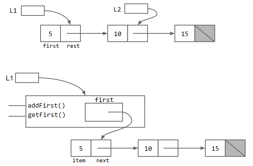

public class IntNode {
    public int item;
    public IntNode next;

    public IntNode(int i,IntNode n){
        item = i;
        next=n;
    }
}
public class SLList{
    public IntNode first;

    public SLList(int x){
        first = new IntNode(x,null);
    }

    public static void main(String[] args) {
        SLList L= new SLList(10); //这样就不必用空值了
    }
}

嵌套类

如果你没有使用外部类的任何实例成员，则将嵌套类设为静态。

public class SLList {
       public static class IntNode {
		如果嵌套类不需要使用 SLList 的任何实例方法或变量，则可以声明嵌套类 static
            public int item;
            public IntNode next;
            public IntNode(int i, IntNode n) {
                item = i;
                next = n;
            }
       }

       private IntNode first;

递归调用 size 在 IntList 中很简单： return 1 + this.rest.size() 。但对于 SLList ，这种方法没有意义， SLList 没有 rest 变量。所以要used with middleman classes

private static int size(IntNode p){
        if(p.next==null){
            return 1;
        }
        return 1+size(p.next);
    }
    public int size(){
        return size(first);
    }

方法1.都命名为 size ，在 Java 中这是允许的，因为它们的参数不同。我们说具有相同名称但不同签名的两个方法是重载的。

方法2：在 IntNode 类本身创建一个非静态辅助方法。

缓存

增加一个size变量，这样检索更快

public class SLList {
    ... /* IntNode declaration omitted. */
    private IntNode first;
    private int size;
    
    public SLList(int x) {
        first = new IntNode(x, null);
        size = 1;
    }
    public void addFirst(int x) {
        first = new IntNode(x, first);
        size += 1;
    }

    public int size() {
        return size;
    }
}

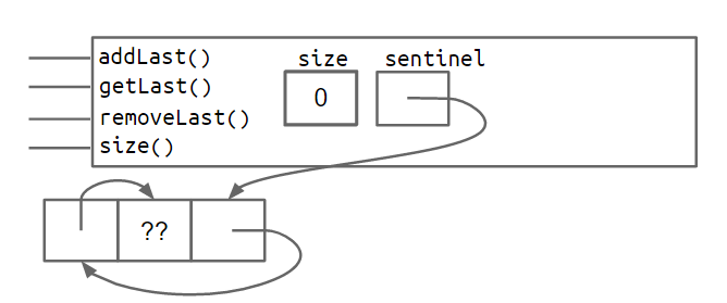
哨兵节点

private IntNode sentinel;
    private int size;

    public SLList() {
        sentinel = new IntNode(-1, null);
        size = 0;
    }

    public SLList(int x) {
        sentinel = new IntNode(-1, null);
        sentinel.next= new IntNode(x,null);
        size = 1;
    }

    public void addFirst(int x) {
        sentinel.next = new IntNode(x, sentinel.next);//sentinel永远指向同一个
        size += 1;
    }

    public int getFirst() {
        return sentinel.next.item;
    }
	public void addLast(int x) {
        size = size+1;

        IntNode p=sentinel;
        while(p.next!=null){
            p=p.next;
        }
        p.next=new IntNode(x,null);
    }

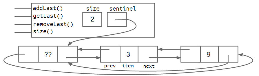
2.3双向链表

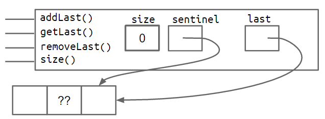
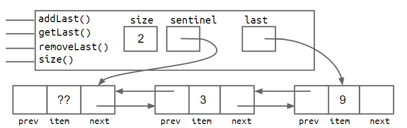
问题：last 指针有时指向哨兵节点，有时指向实际节点。

一种解决方案是在链表末尾添加第二个哨兵节点。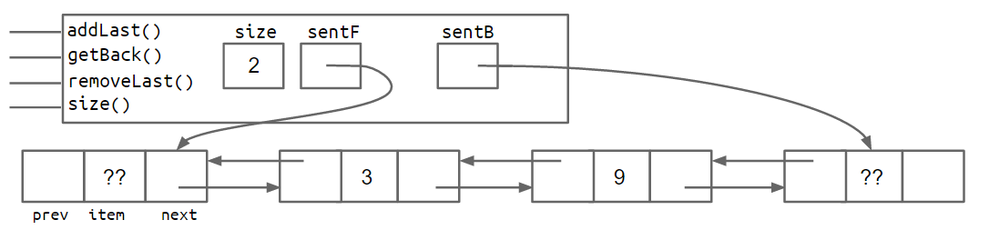

另一种方法是实现一个循环列表，其中前后指针共享同一个哨兵节点。

泛型

public class Printer <>{
    T thingToPrint;
    public Printer(T thingToPrint){
        this.thingToPrint = thingToPrint;
    }
    public void print(){
        System.out.println(thingToPrint);
    }
}

public class GenericsExample{
	public static void main(String[] args){
		Printer<Integer>printer = new Printer<>(23);
		printer.print();
	}
}

实例化:

DLList<String> d2 = new DLList<>("hello");
d2.addLast("world");

int:Integer double:Double char:Character boolean:Boolean long:Long

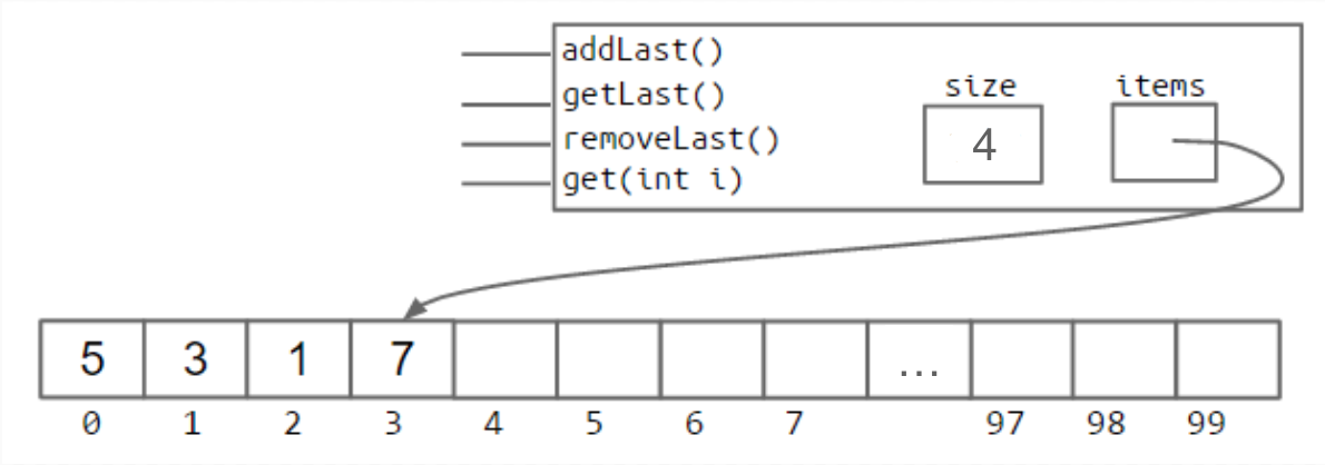
2.4数组

• x = new int[3];
• y = new int[]{1, 2, 3, 4, 5};
• int[] z = {9, 10, 11, 12, 13};`

System.arraycopy(b, 0, x, 3, 2);
原数组b，原数组从0开始，目标数组x，目标数组从第3项开始，2项要复制
等同于 Python 中的 x[3:5] = b[0:2]

Resizing Arrays调整数组大小

仅仅是加了项，创建副本：

int[] a = new int[size + 1];
System.arraycopy(items, 0, a, 0, size);
a[size] = 11;
items = a;
size = size + 1;

这样用＋太慢，而且当RFACTOR太大又占用空间

public void insertBack(int x) {
    if (size == items.length) {
           resize(size + RFACTOR);
    }
    items[size] = x;
    size += 1;
}

可以这样调整大小：

public void insertBack(int x) {
    if (size == items.length) {
           resize(size * RFACTOR);
    }
    items[size] = x;
    size += 1;
}

我们定义一个“使用率”R，它等于列表的大小除以 items 数组长度。比如下图：使用率为0.04

在一个典型实现中，当 R 降至 0.25 以下时，我们将数组大小减半。

3.1JUnit 测试

public class TestSort {
    /** Tests the sort method of the Sort class. */
    public static void testSort() {
        String[] input = {"i", "have", "an", "egg"};
        String[] expected = {"an", "egg", "have", "i"};
        Sort.sort(input);
        for (int i = 0; i < input.length; i += 1) {
            if (!input[i].equals(expected[i])) {
                System.out.println("Mismatch in position " + i + ", expected: " + expected + ", but got: " + input[i] + ".");
                break;
            }
        }
    }
//这样输出过于繁琐
    public static void main(String[] args) {
        testSort();
    }
}

org.junit 库提供了一些有助于简化测试编写的实用方法和功能

public static void testSort() {
    String[] input = {"i", "have", "an", "egg"};
    String[] expected = {"an", "egg", "have", "i"};
    Sort.sort(input);
    org.junit.Assert.assertArrayEquals(expected, input);
}

怎么比较字符串：

str1.compareTo(str2) method will return a negative number if str1 < str2, 0 if they are equal, and a positive number if str1 > str2

递归时用私有辅助方法

/** Sorts strings destructively. */
public static void sort(String[] x) { 
   int smallestIndex = findSmallest(x);
   swap(x, 0, smallestIndex);
   sort(x[1:])//但是java并没有切片功能，×
}

private static void sort(String[] x, int start) { //有了额外的参数 start
   int smallestIndex = findSmallest(x);
   swap(x, start, smallestIndex);
   sort(x, start + 1);
}//现在我们设置正确的原始调用
public static void sort(String[] x) { 
   sort(x, 0);
}

4.1继承，实现

重载

让某方法也适用于 AList

把public static String longest(SLList<String> list)改成
public static String longest(AList<String> list)

Java 会根据你提供的参数类型来知道运行哪个。如果你提供 AList，它将调用 AList 方法。

接口

首先如果 SLList 是 List61B 的下义词，则 SLList 类是 List61B 类的子类，而 List61B 类是 SLList 类的超类。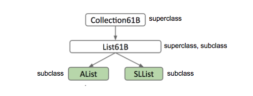

表达这个层次结构的步骤：

• 第一步：定义一个用于通用列表超类型的类型 – 我们将选择名称 List61B。
• 第二步：指定 SLList 和 AList 是该类型的下位词。

public interface List61B<Item> {//这是List61B接口
    public void addFirst(Item x);
    public void add Last(Item y);
    public Item getFirst();
    public Item getLast();
    public Item removeLast();
    public Item get(int i);
    public void insert(Item x, int position);
    public int size();
}
//现在指定 AList 和 SLList 是 List61B 类的下位词
public class AList<Item> implements List61B<Item>{...}

覆盖Override

@Override
方便编译，检查拼写错误

Interface Inheritance 接口继承

接口继承指的是子类继承父类所有方法/行为的关系。例如，在“同义词和上位词”部分中我们定义的 List61B 类，接口包括所有方法签名，但不包括实现。具体实现由子类提供。

这种继承是多代的。这意味着如果我们有一个像图 4.1.1 中那样的长序列的超类/子类关系，AList 不仅继承自 List61B 的方法，还继承自它上面的所有其他类，一直到最高超类，即 AList 继承自 Collection。

Implementation Inheritance 实现继承

关键字default

如果我们在 List61B定义这个方法
default public void print() {
    for (int i = 0; i < size(); i += 1) {
        System.out.print(get(i) + " ");
    }
    System.out.println();
}
然后，所有实现 List61B 类的都可以使用该方法！

接口继承（是什么）：简单地说明子类应该能够做什么。

• 所有列表都应该能够打印自身，它们如何做到这一点由它们自己决定。

实现继承（如何）：告诉子类它们应该如何表现。

• 列表应该以这种方式打印出来：先按顺序获取每个元素，然后打印它们。

4.2Extend

继承允许子类重用已定义类中的代码。现在我们定义 RotatingSLList 类，使其继承自 SLList。

我们可以使用 extends 关键字在类头中设置这种继承关系，如下所示：

public class RotatingSLList<Item> extends SLList<Item>

构造函数不会被继承，私有成员不能被子类直接访问。

public class VengefulSLList<Item> extends SLList<Item> {
    SLList<Item> deletedItems;/* =new SLList<Item>();效果与下面相同*/

    public VengefulSLList() {
        deletedItems = new SLList<Item>();
    }

    @Override
    public Item removeLast() {
        Item x = super.removeLast();/***调用父类的方法*/
        deletedItems.addLast(x);
        return x;
    }

    /** Prints deleted items. */
    public void printLostItems() {
        deletedItems.print();
    }
}

构造函数不可继承:

比如有两个类：

public class Human {...}
public class TA extends Human {...}
如果运行 TA Christine = new TA();
首先，必须创建一个人类。然后，那个人类可以被赋予助教的品质。在没有首先创建人类的情况下构建助教是没有意义的。

因此，我们可以显式地调用超类的构造函数，使用 super 关键字：
public VengefulSLList() {
    super();
    deletedItems = new SLList<Item>();
}
public VengefulSLList(Item x) {
    super(x);
    deletedItems = new SLList<Item>();
}

The Object Class

Interface don’t extend Object.

Object 类提供了很多基本的方法，例如toString() ， equals() 等

抽象屏障

隐藏用户不需要知道的东西

Type Checking and Casting

静态类型，动态类型

记住，编译器根据对象的静态类型确定某事物是否有效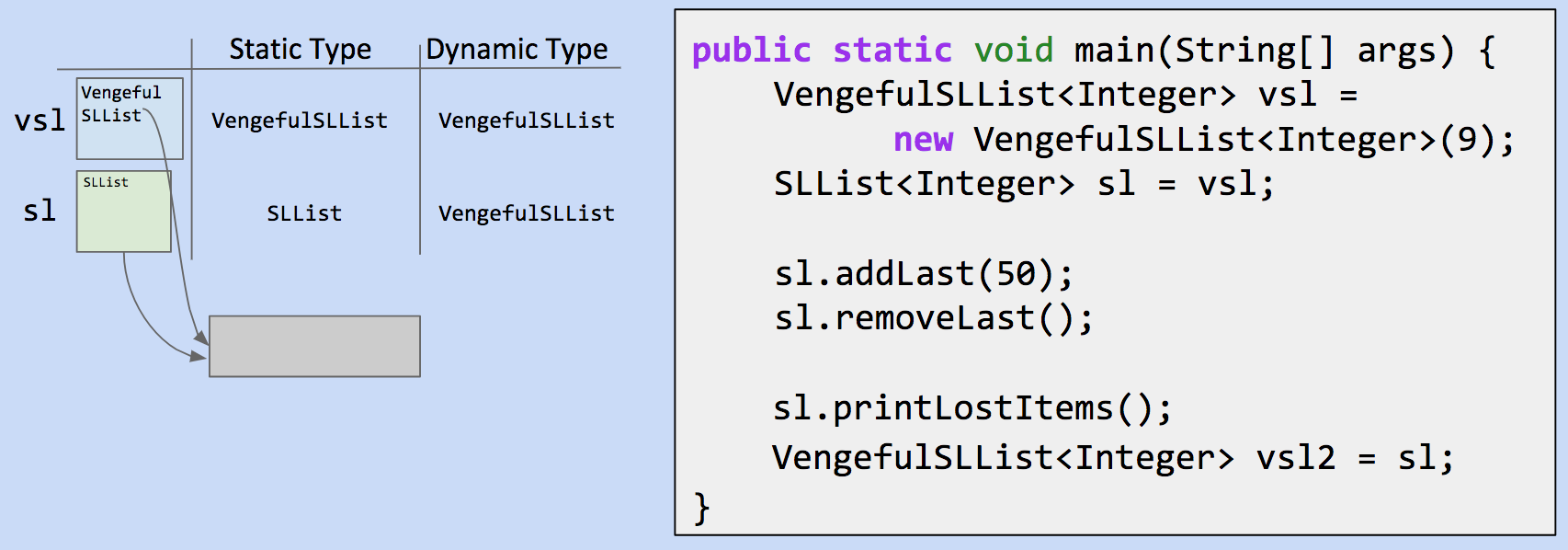倒数第二行：由于 sl 的静态类型为 SLList，而 printLostItems 未在 SLList 类中定义，即使 sl 的运行时类型为 VengefulSLList，代码也不允许运行。

倒数第一行：一般来说，编译器只允许基于编译时类型的调用和赋值。由于编译器只看到 sl 的静态类型是 SLList，它不会允许一个 VengefulSLList “容器”来持有它。

Expressions

SLList<Integer> sl = new VengefulSLList<Integer>();//正确
上述表达式的右侧编译时类型为 VengefulSLList。编译器检查以确保 VengefulSLList“是”SLList 的子类，并允许这种赋值

VengefulSLList<Integer> vsl = new SLList<Integer>();//编译错误

Casting

类型转换

Poodle largerPoodle = (Poodle) maxDog(frank, frankJr); // compiles! Right hand side has compile-time type Poodle after casting

类型转换的风险

Poodle frank = new Poodle("Frank", 5);
Malamute frankSr = new Malamute("Frank Sr.", 100);

Poodle largerPoodle = (Poodle) maxDog(frank, frankSr); // runtime exception!

在这种情况下，我们比较了一只贵宾犬和一只马尔穆特犬。没有类型转换，编译器通常不会允许调用 maxDog 进行编译，因为右侧的编译时类型将是 Dog，而不是 Poodle。然而，类型转换允许这段代码通过，当 maxDog 在运行时返回马尔穆特犬，并且我们尝试将马尔穆特犬转换为贵宾犬时，我们会遇到运行时异常 - 一个 ClassCastException

Inheritance Cheatsheet

VengefulSLList extends SLList 表示 VengefulSLList 是 SLList ，并继承所有 SLList 的成员：

Higher Order Functions

//编写一个接口，定义任何接受整数并返回整数的函数 - 一个 IntUnaryFunction 。

public interface IntUnaryFunction {
    int apply(int x);
}

//现在我们可以编写一个类来表示一个具体函数。让我们编写一个函数，它接受一个整数并返回该整数的 10 倍。
public class TenX implements IntUnaryFunction {
    /* Returns ten times the argument. */
    public int apply(int x) {
        return 10 * x;
    }
}
//在这个阶段，我们已经用 Java 实现了 Python 中的 tenX 函数的等价功能。现在我们来写 do_twice 。
public static int do_twice(IntUnaryFunction f, int x) {
    return f.apply(f.apply(x));
}

//Java 中调用 print(do_twice(tenX, 2)) 的代码如下：
System.out.println(do_twice(new TenX(), 2));

4.3Subtype Polymorphism

子类型多态。为不同类型的实体提供单一接口

1. Explicit HoF Approach 显式 HoF 方法

def print_larger(x, y, compare, stringify):
    if compare(x, y):
        return stringify(x)
    return stringify(y)

1. Subtype Polymorphism Approach
   子类型多态方法

def print_larger(x, y):
    if x.largerThan(y):
        return x.str()
    return y.str()

问题背景：

public static Object max(Object[] items) {
    int maxDex = 0;
    for (int i = 0; i < items.length; i += 1) {
        if (items[i] > items[maxDex]) {//  Complilation Error
            maxDex = i;
        }
    }
    return items[maxDex];
}
public static void main(String[] args) {
    Dog[] dogs = {new Dog("Elyse", 3), new Dog("Sture", 9), new Dog("Benjamin", 15)};
    Dog maxDog = (Dog) max(dogs);
    maxDog.bark();
}//放弃实现一个通用的 max 函数
public static Dog maxDog(Dog[] dogs) {
    if (dogs == null || dogs.length == 0) {
        return null;
    }
    Dog maxDog = dogs[0];
    for (Dog d : dogs) {
        if (d.size > maxDog.size) { //
            maxDog = d;
        }
    }
    return maxDog;
}
基本问题是对象无法与 > 进行比较。这很有道理，Java 如何知道应该使用对象的字符串表示、大小还是其他指标来进行比较呢？在 Python 或 C++中， > 运算符的作用方式可以根据应用到的不同类型进行重新定义。不幸的是，Java 没有这种能力。相反，我们转向接口继承来帮助我们。

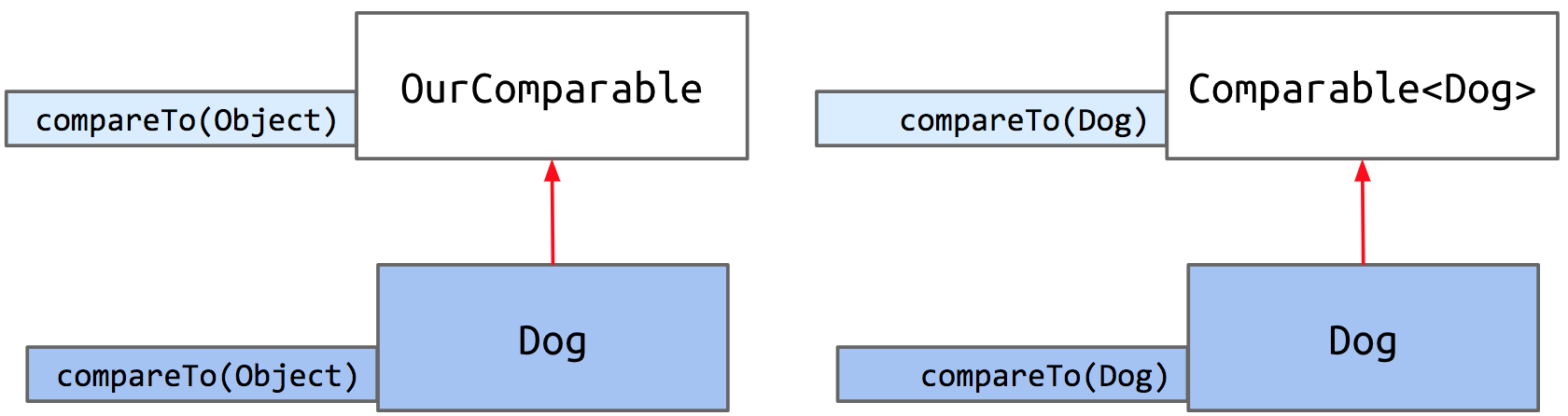
创建一个接口,确保任何实现类，如 Dog，都包含一个比较方法,将其称为 compareTo。

public interface OurComparable{
    public int compareTo(Object o);
}//define its behavior like so:
//Return -1 if this < o. //Return 0 if this equals o. //Return 1 if this > o.

现在我们已经创建了 OurComparable 接口，我们可以要求我们的 Dog 类实现 compareTo 方法。首先，我们将 Dog 类的类头改为包含 implements OurComparable ，然后根据其定义的行为编写 compareTo 方法。

Comparables

OurComparable 接口我们已经构建完成，它能够工作，但并不完美。以下是它的一些问题：

• 尴尬的对象转换
• 我们编造了它。
  • 当前没有现有类实现 OurComparable（例如 String 等。）
  • 当前没有现有类使用 OurComparable（例如，没有使用 OurComparable 的内置 max 函数）

利用一个已存在的接口，称为 Comparable。

Comparable<T> 表示它接受一个泛型类型。这将帮助我们避免将对象强制转换为特定类型

现在，我们将重写 Dog 类以实现 Comparable 接口，确保更新泛型类型 `T` 为 Dog
public class Dog implements Comparable<Dog> {
    ...
    public int compareTo(Dog uddaDog) {
        return this.size - uddaDog.size;
    }
}

不再使用我们亲自创建的接口 OurComparable ，现在使用真实的内置接口 Comparable

Comparator

作为一个例子，狗的自然排序，正如我们之前所述，是根据体型值来定义的。如果我们想以不同于它们自然排序的方式对狗进行排序，比如按照它们名字的字母顺序排序呢？

Java 实现这种方式是通过使用 Comparator 的。由于比较器是一个对象，我们将通过在 Dog 内部编写一个实现 Comparator 接口的嵌套类来使用 Comparator 。

public interface Comparator<T> {
    int compare(T o1, T o2);
}

import java.util.Comparator;
public class Dog implements Comparable<Dog> {
    ...
    public int compareTo(Dog uddaDog) {
        return this.size - uddaDog.size;
    }
    private static class NameComparator implements Comparator<Dog> {
        public int compare(Dog a, Dog b) {
            return a.name.compareTo(b.name);
        }
    }
    public static Comparator<Dog> getNameComparator() {
        return new NameComparator();
    }
}

上述代码相当于c++的运算符重载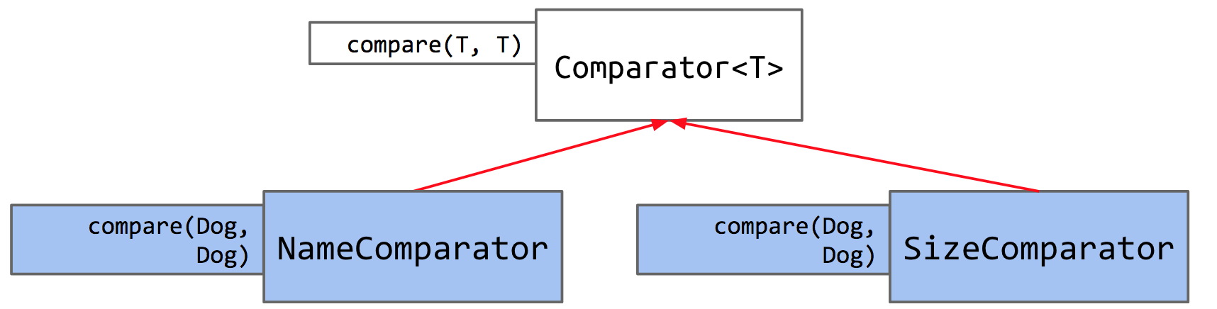

我们有一个内置的 Comparator 接口，我们可以实现它来定义自己的比较器（ NameComparator ， SizeComparator 等）

6.2Throwing Exceptions

public void add(T x) {
    if (x == null) {
        throw new IllegalArgumentException("can't add null");
    }
    if (contains(x)) {
        return;
    }
    items[size] = x;
    size += 1;
}

throw 关键字相当于 python里的raise

6.3Iteration

Set<String> s = new HashSet<>();
...
for (String city : s) {
    ...
}

The above code translates to:

Set<String> s = new HashSet<>();
...
Iterator<String> seer = s.iterator();
while (seer.hasNext()) {
    String city = seer.next();
    ...
}

public Iterator<E> iterator();

Now, we can use that object to loop through all the entries in our list:

List<Integer> friends = new ArrayList<Integer>();
...
Iterator<Integer> seer = friends.iterator();

while (seer.hasNext()) {
System.out.println(seer.next());
}

Implementing Iterators

列表接口扩展了可迭代接口，继承了抽象的 iterator()方法。（实际上，列表扩展了集合，集合又扩展了可迭代接口，但这样理解起来更简单。）

public interface Iterable<T> {
    Iterator<T> iterator();
}
public interface List<T> extends Iterable<T>{
    ...
}

接下来，编译器检查迭代器是否有 hasNext() 和 next() 。迭代器接口明确指定了这些抽象方法：

public interface Iterator<T> {
    boolean hasNext();
    T next();
}

特定类将实现它们自己的接口方法的迭代行为。

我们将向我们的 ArrayMap 类添加通过键进行迭代的特性。首先，我们编写一个新的类，名为 ArraySetIterator，它嵌套在 ArraySet 内部：

private class ArraySetIterator implements Iterator<T> {
    private int wizPos;

    public ArraySetIterator() {
        wizPos = 0;
    }

    public boolean hasNext() {
        return wizPos < size;
    }

    public T next() {
        T returnItem = items[wizPos];
        wizPos += 1;
        return returnItem;
    }
}

此 ArraySetIterator 实现了一个 hasNext() 方法和一个 next() 方法，使用 wizPos 位置作为索引来跟踪其在数组中的位置。

现在我们有了适当的方法，我们可以使用 ArraySetIterator 遍历 ArrayMap：

ArraySet<Integer> aset = new ArraySet<>();
aset.add(5);
aset.add(23);
aset.add(42);

Iterator<Integer> iter = aset.iterator();

while(iter.hasNext()) {
    System.out.println(iter.next());
}

我们仍然希望能够支持增强型 for 循环，以使我们的调用更简洁。因此，我们需要让 ArrayMap 实现 Iterable 接口。Iterable 接口的基本方法是 iterator() ，它为该类返回一个 Iterator 对象。我们只需返回我们刚刚编写的 ArraySetIterator 的一个实例即可！

public Iterator<T> iterator() {
    return new ArraySetIterator();
}

现在我们可以使用增强型 for 循环与我们的 ArrraySet !

ArraySet<Integer> aset = new ArraySet<>();
...
for (int i : aset) {
    System.out.println(i);
}

Object Methods

所有类都继承自根 Object 类

toString()

默认的 Object 类的 toString() 方法打印对象在内存中的位置。这是一个十六进制字符串。像 Arraylist 和 java 数组这样的类有自己的 toString() 方法重写版本。这就是为什么，当你处理和编写 Arraylist 的测试时，错误总是以这种格式（1，2，3，4）返回列表，而不是返回内存位置。

对于我们自己编写的类，如 ArrayDeque 、 LinkedListDeque 等，如果我们想以可读的格式查看打印的对象，则需要提供自己的 toString() 方法。

import java.util.Iterator;
public class ArraySet<T> implements Iterable<T> {
    private T[] items;
    private int size; // the next item to be added will be at position size
    public ArraySet() {
        items = (T[]) new Object[100];
        size = 0;
    }
    ```
    @Override
    public String toString() {
        StringBuilder returnSB = new StringBuilder("{");
        for (int i=0;i<size-1;i+=1){
            returnSB.append(items[i].toStirng());
            returnSB.append(", ");
        }
        returnSB.append(items[size-1]);
        returnSB.append("}");
        return returnSB.toString();
    }
    @Override
    public boolean equals(Object other) {
        if (this == other){
            return true;
        }
        if(other ==null){
            return false;
        }
        if(other.getClass()!=this.getClass()){
            return false;
        }
        ArraySet<T> o = (ArraySet<T>)other;
        if(o.size()!=this.size()){
            return false;
        }
        for(T item:this){
            if(!o.contains(item)){
                return false;
            }
        }
        return true;
    }
    public static void main(String[] args) {
        ArraySet<Integer> aset = new ArraySet<>();
        aset.add(5);aset.add(23);aset.add(42);
        //iteration
        for (int i : aset) {
            System.out.println(i);
        }
        //toString
        System.out.println(aset);
        //equals
        ArraySet<Integer> aset2 = new ArraySet<>();
        aset2.add(5); aset2.add(23);aset2.add(42);
        System.out.println(aset.equals(aset2));System.out.println(aset.equals(null));
        System.out.println(aset.equals("fish")); System.out.println(aset.equals(aset));
}

equals()

Java 中 equals() 和 == 有不同的行为。 == 检查两个对象是否实际上是同一个内存中的对象。记住，按值传递！ == 检查两个盒子是否包含相同的东西。对于原始类型，这意味着检查值是否相等。对于对象，这意味着检查地址/指针是否相等。

Doge fido = new Doge(5, "Fido");
      Doge doggo = new Doge(6, "Doggo");
      Doge fidoTwin = new Doge(5, "Fido");
      Doge fidoRealTwin = fido;
      
fido 和 fidoTwin 不被视为 == ，因为它们指向不同的对象。

equals(Object o)

是 Object 中的一个方法，默认情况下它像 == 一样工作，检查 this 的内存地址是否与 o 相同。然而，我们可以重写它来定义我们想要的任何相等性。例如，对于两个 ArrayList 被认为是相等的，它们只需要具有相同顺序的相同元素即可。

Java 中 equals 方法的规则：当重写一个 .equals() 方法时，有时可能比看起来更复杂。在实现您的 .equals() 方法时，以下是一些需要遵守的规则：

1.) equals 必须是一个等价关系

• reflexive自反: x.equals(x) 为真
• symmetric对称: x.equals(y) if and only if y.equals(x)
• transitive: 及物： x.equals(y) 和 y.equals(z) 蕴含 x.equals(z)

2.) 必须传递一个对象参数，以覆盖原始的 .equals() 方法

3.) 如果 x.equals(y) ，则只要 x 和 y 保持不变： x 必须继续等于 y

4.) 对于 null， x.equals(null) 必须为假

Efficient Programming

编写一个使用链表作为其底层数据结构的 Stack 类。您只需要实现一个函数：push(Item x)。确保使用”Item”作为泛型类型使该类通用！

1)使用拓展 public class ExtensionStack<Item> extends LinkedList<Item> {
    public void push(Item x){
        add(x);
    }
}
2)使用委托 创建一个链表对象并调用其方法以实现其目标 
public class DelegationStack<Item> {
    private LinkedList<Item> L = new LinkedList<Item>();
    public void push(Item x) {
        L.add(x);
    }
}
3)这种方法与之前的方法类似，除了它可以使用实现 List 接口的任何类（如 LinkedList、ArrayList 等）。
public class StackAdapter<Item> {
    private List L;
    public StackAdapter(List<Item> worker){
        L = worker;
    }
    public void push(Item x){
        L.add(x);
    }
}
//委托是通过传递一个类来完成的，而扩展被定义为继承

不相交集合（并查集）

假设我们有四个元素，我们将它们称为 A、B、C、D。一开始，每个元素都在自己的集合中。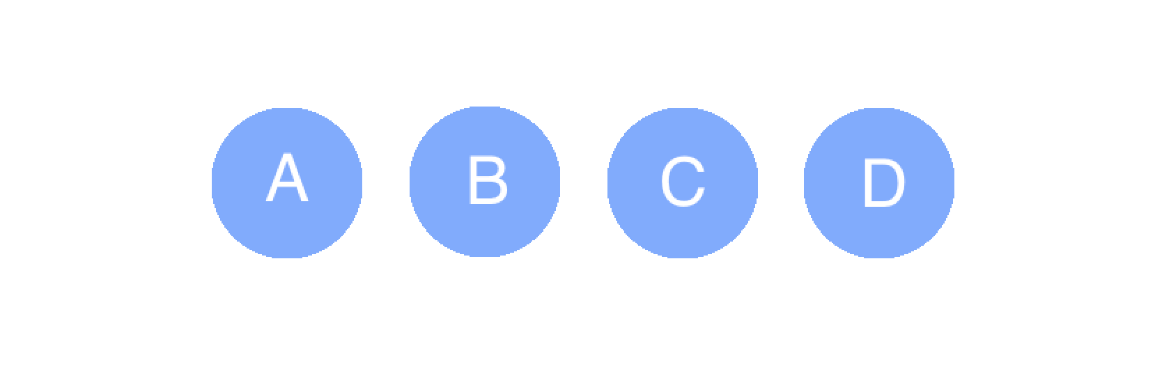

在调用 connect(A, B) 后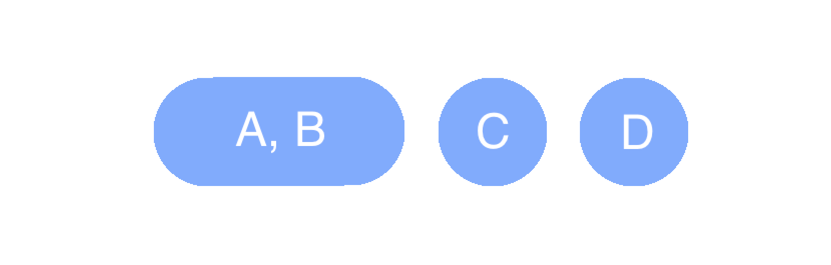

isConnected(A, B) -> true
isConnected(A, C) -> false

我们正式定义我们的 DisjointSets:

public interface DisjointSets {
    void connect (int p,int q);
    
    boolean isConnected(int p,int q);
}

Quick Find

考虑使用一个整数数组作为另一种方法。····数组索引代表我们集合的元素。索引处的值是该集合所属的编号。

例如：表示 {0, 1, 2, 4}, {3, 5}, {6} 为

public class QuickFindDS implements DisjointSets {
    private int[] id;
    /* Θ(N) */
    public QuickFindDS(int N){
        id = new int[N];
        for (int i = 0; i < N; i++){
            id[i] = i;
        }
    }
    /* need to iterate through the array => Θ(N) */
    public void connect(int p, int q){
        int pid = id[p];
        int qid = id[q];
        for (int i = 0; i < id.length; i++){
            if (id[i] == pid){
                id[i] = qid;
            }
        }
    }
    /* Θ(1) */
    public boolean isConnected(int p, int q){
        return (id[p] == id[q]);
    }
}

Quick Union

我们给每个项目分配其父项的索引。如果一个项目没有父项，那么它是一个’root’，我们给它分配一个负值。例如，我们表示 {0, 1, 2, 4}, {3, 5}, {6} 为：：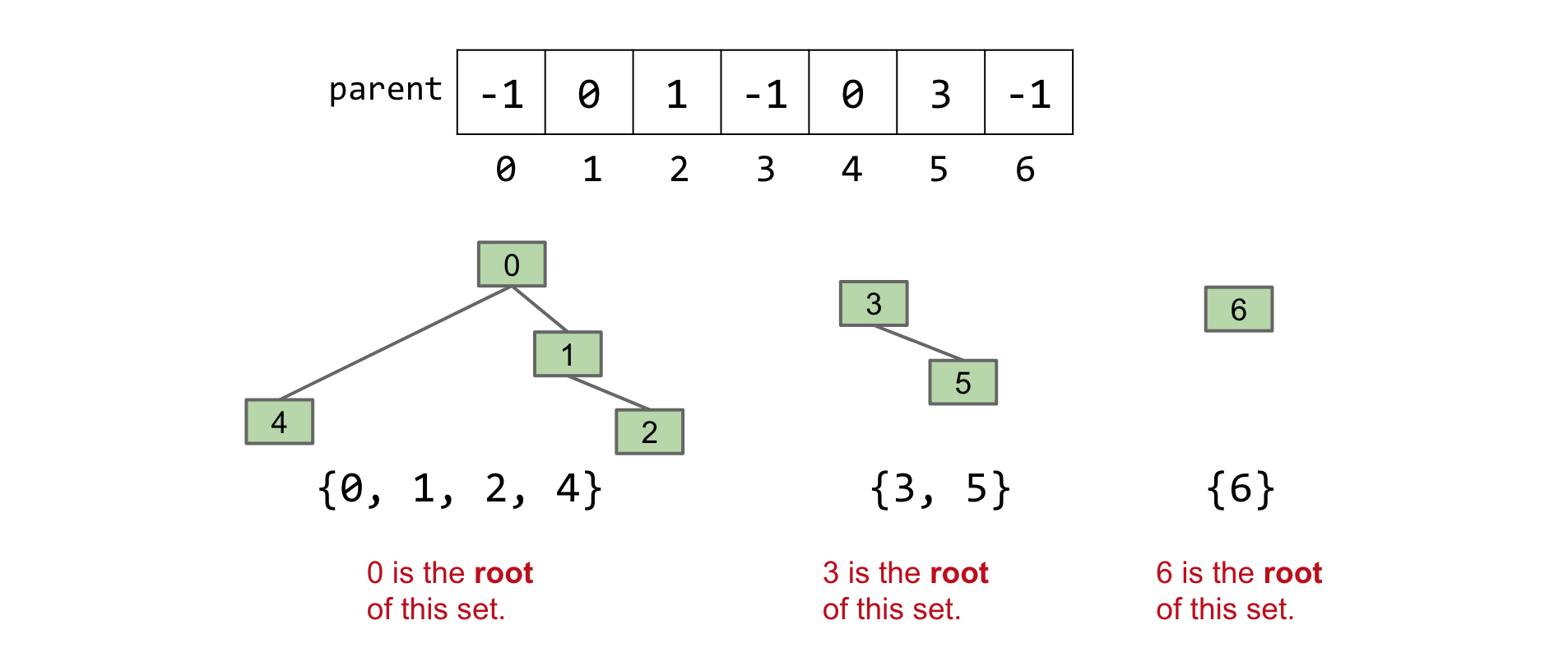

对于 QuickUnion，我们定义一个辅助函数 find(int item) ，它返回树 item 所在的根。

public class QuickUnionDS implements DisjointSets {
    private int[] parent;
    public QuickUnionDS(int num) {
        parent = new int[num];
        for (int i = 0; i < num; i++) {
            parent[i] = i;
        }
    }
    private int find(int p) {
        while (parent[p] >= 0) {
            p = parent[p];
        }
        return p;
    }
    @Override
    public void connect(int p, int q) {
        int i = find(p);
        int j= find(q);
        parent[i] = j;
    }
    @Override
    public boolean isConnected(int p, int q) {
        return find(p) == find(q);
    }
}

Weighted Quick Union (WQU)加权快速并查集

新规则：每次我们调用 connect 时，我们总是将较小树的根连接到较大树上。遵循此规则将使树的最大高度为 logN ，其中 N 是我们并查集中元素的数量。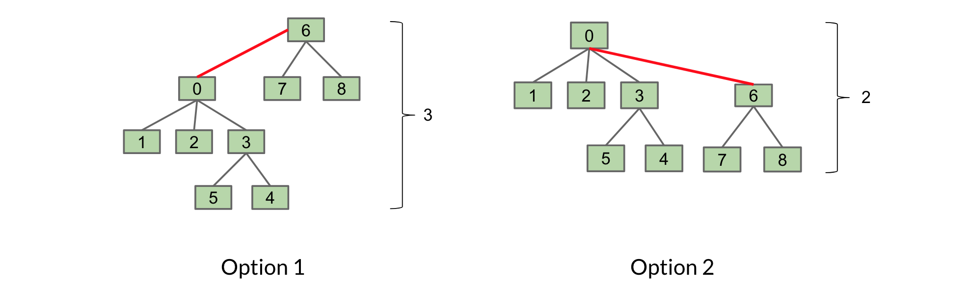选第2种

Weighted Quick Union with Path Compression

路径压缩的优化思想是：

• 在 Find 操作中，将查找路径上的所有节点直接连接到根节点。
• 这样可以进一步减少树的高度，使得后续的 Find 操作更快。

Binary Search二分查找

static int binarySearch(String[] sorts,String x,int lo,int hi){
    if(lo>hi) return -1;
	int m=(lo+hi)/2;
	int cmp=x.compareTo(sorted[m]);
	if(cmp<0) return binarySearch(sorts,x,lo,m-1);
	else if(cmp>0)return binarySearch(sorts,x,m+1,hi);
	else return m;
}

时间复杂度：Θ(logN)

Merge Sort归并排序

runtime: N logN

ADTs

几个有用的 ADT：

• 非交集集合，映射，集合，列表。
• Java 提供了 Map、Set、List 接口，以及几个实现。

Trees

Binary Search Trees

• 每个左子树中的键都小于 X 的键。每个右子树中的键都大于 X 的键。

约束：任意两个节点之间只有一条路径。 传递性：p<q and q<r imply p<r 反对称性： Exactly one of p<q and q<p are true

不能有重复，比如2个dog

这里是我们将在本模块中使用的二叉搜索树（BST）类：

private class BST<Key> {
    private Key key;
    private BST left;
    private BST right;

    public BST(Key key, BST left, BST Right) {
        this.key = key;
        this.left = left;
        this.right = right;
    }

    public BST(Key key) {
        this.key = key;
    }
}

Binary Search Tree Operations

Search

static BST find(BST T,Key sk){
    if (T==null){
        return null;
    }
    if(sk.equals(T.key)){
        return T;
    }
    else if (sk< T.key){
        return find(T.left,sk);
    }
    else return find(T.right,sk);
}

Insert

static BST insert(BST T,Key ik){
	if(T==null){
		return new BST(ik);
	}
    if(ik<T.key){
        T.left=insert(T.left,ik);
    }
    else if(ik>T.key){
        T.right=insert(T.right,ik);
    }
    return T;
}

Delete

让我们将这个问题分解为三个类别：

• 我们要删除的节点没有子节点 ：直接删
• 有 1 个子节点 ：子承父业
• 有 2 个子节点 ：选择一个新的节点来替换被删除的节点。只需取左子树最右边的节点或右子树最左边的节点即可（称为 Hibbard 删除）

Balanced Search Trees

Worst case: Θ(N)Θ(N)

Best-case: Θ(logN)Θ(logN) (where N is number of nodes in the tree)

Some terminology for BST performance:

• depth: the number of links between a node and the root.
• height: the lowest depth of a tree.
• average depth: average of the total depths in the tree.

The height of the tree determines the worst-case runtime, because in the worst case the node we are looking for is at the bottom of the tree.

The average depth determines the average-case runtime.

B-Trees

Insertion Process 插入过程

The process of adding a node to a 2-3-4 tree is:
添加节点到 2-3-4 树的过程是：

1. 我们仍然总是插入到叶节点，所以取要插入的节点并带着它遍历树，根据要插入的节点是否大于或小于每个节点中的项来决定是向左还是向右移动。
2. 在将节点添加到叶节点后，如果新节点有 4 个节点，则弹出中间左节点并相应地重新排列子节点。
3. 如果这导致父节点有 4 个节点，那么再次弹出中间左节点，相应地重新排列子节点。
4. 重复此过程，直到父节点可以容纳或到达根节点。
   对于 2-3 树，执行相同的过程，除了在 3 元素节点中向上推送中间节点。

B-Tree invariants

B 树具有以下有用的不变性：

• 所有叶子必须与源头保持相同的距离。
• 一个包含 k 项的非叶节点必须恰好有 k+1 个子节点。

runtime:总运行时间是 O(logN)

Rotating Trees

旋转的正式定义是：

rotateLeft(G): Let x be the right child of G. Make G the new left child of x.
rotateRight(G): Let x be the left child of G. Make G the new right child of x.

以下是节点 G 左旋操作发生情况的图形描述：
G 的右子树 P 与 G 合并，并带上其子树。然后 P 将其左子树传递给 G，G 向下移动到左边成为 P 的左子树。

相关代码：

private Node rotateRight(Node h) {
    Node x = h.left;
    h.left = x.right;
    x.right = h;
    return x;
}

private Node rotateLeft(Node h) {
    Node x = h.right;
    h.right = x.left;
    x.left = h;
    return x;
}

Red-Black Trees

任意选择将左元素作为右元素的子元素。这导致了一棵左倾树。我们通过将其染成红色来证明链接是一个粘合链接。正常链接是黑色的。因此，我们称这些结构为左倾红黑树（LLRB）。

左倾红黑树与 2-3 树一一对应。每个 2-3 树都有一个唯一的左倾红黑树与之关联。至于 2-3-4 树，它们与标准红黑树保持对应关系。

Properties of LLRB’s

LLRB 的属性如下：

• 1-1 对应于 2-3 树。
• 没有节点有 2 个红色链接。
• 没有红色右链。
• 每条从根到叶子的路径都有相同数量的黑色链接（因为 2-3 树到每个叶子的链接数量相同）。
• 高度不超过对应 2-3 树 2 倍的高度。

Here is a summary of all the operations:
When inserting: Use a red link.
If there is aright leaning “3-node”, we have a Left Leaning Violation

• • Rotate left the appropriate node to fix.
• If there are two consecutive left links, we have an incorrect 4 Node Violation!
  • Rotate right the appropriate node to fix.
• If there are any nodes with two red children, we have a temporary 4 Node.
  • Color flip the node to emulate the split operation.

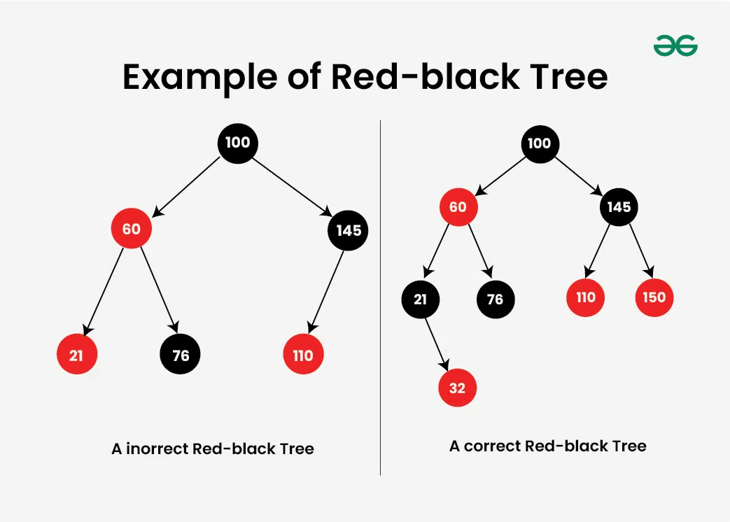
Properties of Red-Black Trees

A Red-Black Tree have the following properties:

1.Node Color: Each node is either red or black.
2.Root Property: The root of the tree is always black.
3.Red Property: Red nodes cannot have red children (no two consecutive red nodes on any path).
4.Black Property: Every path from a node to its descendant null nodes (leaves) has the same number of black nodes.
5.Leaf Property: All leaves (NIL nodes) are black.

Runtime

Because a left-leaning red-black tree has a 1-1 correspondence with a 2-3 tree and will always remain within 2x the height of its 2-3 tree, the runtimes of the operations will take logN time.

Here’s the abstracted code for insertion into a LLRB:

private Node put(Node h, Key key, Value val) {
    if (h == null) { return new Node(key, val, RED); }

    int cmp = key.compareTo(h.key);
    if (cmp < 0)      { h.left  = put(h.left,  key, val); }
    else if (cmp > 0) { h.right = put(h.right, key, val); }
    else              { h.val   = val;                    }

    if (isRed(h.right) && !isRed(h.left))      { h = rotateLeft(h);  }
    if (isRed(h.left)  &&  isRed(h.left.left)) { h = rotateRight(h); }
    if (isRed(h.left)  &&  isRed(h.right))     { flipColors(h);      } 

    return h;
}

Hashing

用数组来代替BST,BT,LLRB，index代表数据，true/false代表是否被存储

• 如何适用除数字以外的其他数据？——用 ASCII / Unicode
• 不可避免的冲突？——内部使用 List 结构 取模压空间
• 内存开销巨大？运行时不稳定？——使用限定大小且动态增长的数组！同时进一步改进我们的 Hashcode!

Properties of HashCodes

1. It must be an Integer
2. If we run .hashCode() on an object twice, it should return the same number
3. Two objects that are considered .equal() must have the same hash code.

1. 哈希表的基本工作原理

1. 哈希函数转换
   • 输入项（如键值对）通过哈希函数（hashcode）转换为整数。
   • 通过取模运算（%）将该整数映射到哈希表数组的有效索引位置。
2. 冲突处理
   • 若目标索引为空，创建新链表并将输入项加入其中。
   • 若索引已存在链表，则遍历链表检查重复项。若无重复，将输入项追加至链表末尾。
3. 查询逻辑
   • 计算目标索引，遍历对应链表查找指定项，时间复杂度取决于链表长度。

---

2. 处理性能问题

关键挑战：哈希冲突导致的链表长度不均，影响操作效率。

场景	表现	时间复杂度
最佳情况	所有项均匀分布在 M 个桶中，每桶含 N/M 项	Θ(1)（均摊）
最坏情况	所有项堆积到同一桶中，形成长度为 N 的链表	Θ(N)（退化为链表）

优化策略：

1. 动态扩容哈希表

   • 负载因子（Load Factor）：定义为 N/M（项数/桶数），代表哈希表的空间利用率。

   • 扩容阈值

     ：当负载因子超过预设值（如0.75），触发以下操作：

     • 创建新哈希表，桶数翻倍（2M）。
     • 遍历旧表所有项，按新表大小重新计算索引并迁移（因取模结果可能变化）。

   • 扩容耗时：Θ(N)（需逐项迁移，但插入新表时无需查重，直接链表头部追加，单次操作为 Θ(1)）。

2. 优化哈希码设计

   • 目标：确保不同输入项生成尽可能随机的哈希码，减少冲突概率。
   • 实践建议：
     • 使用小质数作为哈希计算基数（如31），避免因整数溢出导致的系统性冲突。
     • 避免依赖局部特征（如字符串末尾字符），防止相似输入哈希码趋同。

Heaps

堆的基本定义如下：

• 首先是一颗完整的二叉树
• 每个结点的值小于等于其两个子节点的值(当然在求 max 的情况下反过来即可)
• 所有结点尽量左倾

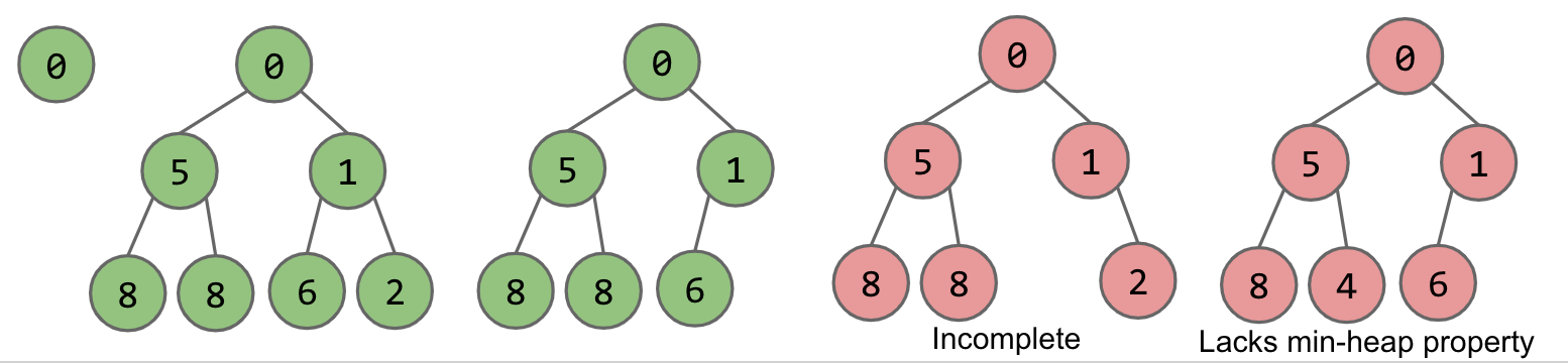
如上图所示：红色的即为不合规的堆
我们关心优先级队列的三种方法是 add ， getSmallest 和 removeSmallest 。

• add: Add to the end of heap temporarily. Swim up the hierarchy to the proper place.
  • Swimming involves swapping nodes if child < parent
• getSmallest: Return the root of the heap (This is guaranteed to be the minimum by our min-heap property
• removeSmallest: Swap the last item in the heap into the root. Sink down the hierarchy to the proper place.
  • Sinking involves swapping nodes if parent > child. Swap with the smallest child to preserve min-heap property

Methods	Ordered Array	Bushy BST	Hash Table	Heap
add	Θ(N)	Θ(logN)	Θ(1)	Θ(logN)
getSmallest	Θ(1)	Θ(logN)	Θ(N)	Θ(1)
removeSmallest	Θ(N)	Θ(logN)	Θ(N)	Θ(logN)

Tree Traversal

has one natural way to iterate through it:

1. Level order traversal.
2. Depth-First traversals –– of which there are three: pre-order, in-order and post-order.

Level Order Traversal（是一种BFS)

一层一层遍历，从第 0 层(即根节点)开始，一步步向后推·······

得到的结果是： D B F A C E G

Depth-First traversals –– of which there are three: pre-order, in-order and post-order.（DFS）

Pre-order Traversal 上， 左右

preOrder(BSTNode x) {
    if (x == null) return;
    print(x.key)
    preOrder(x.left)
    preOrder(x.right)
}

In-order Traversal 左中右

inOrder(BSTNode x) {
    if (x == null) return;    
    inOrder(x.left)
    print(x.key)
    inOrder(x.right)
}

Post-order Traversal 左右中

postOrder(BSTNode x) {
    if (x == null) return;    
    postOrder(x.left)
    postOrder(x.right)
    print(x.key)   
}

DFS伪代码

mark s  // i.e., remember that you visited s already
if (s == t):
    return true;

for child in unmarked_neighbors(s): // if a neighbor is marked, ignore!
    if isconnected(child, t):
        return true;

return false;

BFS伪代码

Initialize the fringe (a queue with the starting vertex) and mark that vertex.
Repeat until fringe is empty:
Remove vertex v from the fringe.
For each unmarked neighbor n of v:
Mark n.
Add n to fringe.
Set edgeTo[n] = v.
Set distTo[n] = distTo[v] + 1.

A fringe is just a term we use for the data structure we are using to store the nodes on the frontier of our traversal’s discovery process (the next nodes it is waiting to look at). For BFS, we use a queue for our fringe.

edgeTo[...] is a map that helps us track how we got to node n; we got to it by following the edge from v to to n.

distTo[...] is a map that helps us track how far n is from the starting vertex. Assuming that each edge is worth a distance of 1, then the distance to n is just one more than the distance to get to v. Why? We can use the way we know how to get to v, then pay one more to arrive at n via the edge that necessarily exists between v and n (it must exist since in the for loop header, n is defined as a neighbor of v).

Representing Graphs

public class Graph {
  public Graph(int V):               // Create empty graph with v vertices
  public void addEdge(int v, int w): // add an edge v-w
  Iterable<Integer> adj(int v):      // vertices adjacent to v
  int V():                           // number of vertices
  int E():                           // number of edges
...

接下来，我们将讨论可以用来表示我们的图的基本数据结构。

Adjacency Matrix 邻接矩阵
我们可以通过使用二维数组来实现这一点。如果连接顶点 s 到 t 的边对应单元格是 1 （表示 true ），则存在一条边连接顶点 s 到 t 。注意，如果图是无向的，邻接矩阵将对角线（从左上角到底右角）将是对称的。

Edge Sets 边集
另一种方法是存储所有边的单个集合。

Adjacency Lists 邻接表

第三种方法是维护一个由顶点编号索引的列表数组。如果从 s 到 t 存在边，则数组索引 s 的列表将包含 t 。

Shortest Paths

19.2 dijkstra

目的：找最短路径树

步骤：

1. 创建一个优先队列。
2. 将 ss 添加到优先队列中，优先级为0 。将所有其他顶点添加到优先队列中，优先级为 ∞ 。
3. 当优先队列不为空时：从优先队列中弹出一个顶点，并松驰从这个顶点出发的所有边。

松弛，即对当前顶点的所有边进行一个距离的检查，如果当前顶点的距离加上该边的权重小于该边另一个顶点的距离，则更新之。这个计算潜在距离、检查是否更好并可能更新的整个过程被称为放松(relax)。

伪代码

def dijkstras(source):
    PQ.add(source, 0)
    For all other vertices, v, PQ.add(v, infinity)
    while PQ is not empty:
        p = PQ.removeSmallest()
        relax(all edges from p)
def relax(edge p,q):
   if q is visited (i.e., q is not in PQ):
       return

   if distTo[p] + weight(edge) < distTo[q]:
       distTo[q] = distTo[p] + w
       edgeTo[q] = p
       PQ.changePriority(q, distTo[q])

19.3 A*

指定源点，指定目标点，求源点到达目标点的最短距离

直观上，Dijkstra 算法从源节点开始（想象源节点是圆的中心。）然后，Dijkstra 算法现在围绕这个点绘制同心圆，半径逐渐增大，并“扫过”这些圆，捕获点。所以，迪杰斯特拉首先访问的是离源点最近的城市，然后是下一个最近的城市。迪杰斯特拉所做的是首先访问所有距离为 1 个单位的城市，然后是距离为 2 个单位的城市，依此类推。

教材演示https://docs.google.com/presentation/d/177bRUTdCa60fjExdr9eO04NHm0MRfPtCzvEup1iMccM/edit#slide=id.g771336078_0_180

让我们稍微修改一下 Dijkstra 算法。在 Dijkstra 算法中，我们使用了 bestKnownDistToV 作为算法中的优先级。这次，我们将使用 +bestKnownDistToV+estimateFromVToGoal 作为我们的启发式函数。

在其他地方学的是：在djikstra 源点->当前点 基础上 变为 源点->当前点(真实距离) +当前点 ->目标点(预估距离)，而我们要写个预估函数，在堆中根据 这个 来排序。

预估函数 要保证 ≤x->终点真实最短距离。有向图不好估计，一般是二维网络直接曼哈顿距离

|x1-x2|+|y1-y2|（只能上下左右情况）

对角线距离 ： max{|x1-x2|,|y1-y2|}（能走斜线情况）

Minimum Spanning Trees

20.1MSTs and Cut Property

cut: 将图中的节点分配到两个非空集合（即我们将每个节点分配到第一集合或第二集合）的分配。

crossing edge:连接一个集合中的节点到另一个集合中的节点的边

Cut Property: given any cut, the minimum weight crossing edge is in the MST.

20.2 Prim and Kruskal

(对不起这部分用了c++的板子写，后面会改回来的)

1. Prim算法（朴素版） → “出圈法”

• 核心逻辑：每次从当前生成树的”外圈”（未加入的顶点集合）中，选择距离生成树最近的顶点加入。

• 操作特点：通过遍历所有未加入顶点，找到与生成树相连的最小权重边（即”出圈”操作）。

  强调从”外圈”顶点中逐步选出最近的顶点加入生成树。

• 时间复杂度：O(n²)

  prim 朴素
  #include<iostream>
  #include<cstring>
  #include<algorithm>
  #include<vector>
  #define inf 1e9
  using namespace std;
  int n,m,a,b,c,ans,cnt;
  const int N =5010;
  struct edge{int v,w;};
  vector<edge> e[N];
  int d[N], vis[N];
  
  bool prim(int s){
      for(int i=0;i<=n;i++)d[i]=inf;
      d[s]=0;
      for(int i=1;i<=n;i++){
          int u=0;
          for(int j=1;j<=n;j++)
              if(!vis[j]&&d[u]>d[j])u=j;
          vis[u]=1;//标记u已出圈
          ans+=d[u];
          if(d[u]!=inf)cnt++;
          for(auto ed: e[u]){
              int v=ed.v,w=ed.w;
              if(d[v]>w)d[v]=w;
          }
      }
      return cnt==n;
  }
  int main()
  {
      cin>>n>>m;
      for(int i=0;i<m;i++){
          cin>>a>>b>>c;
          e[a].push_back({b,c});
          e[b].push_back({a,c});
      }
      if(!prim(1))puts("orz");
      else printf("%d\n",ans);
      return 0;
  }

2. Prim算法（堆优化版） → “出队法”

• 核心逻辑：用优先队列（堆）维护候选边，每次直接取出堆顶的最小权重边。

• 操作特点：通过堆快速获取最小边，避免遍历所有顶点（即”出队”操作）。

  强调从优先队列中不断”出队”最小边。

• 时间复杂度：O(m log m)

  prim -heap
  #include<iostream>
  #include<algorithm>
  #include<cstring>
  #include<queue>
  #define inf 1e9
  using namespace std;
  
  const int N=5010;
  int n,m,a,b,c,ans,cnt;
  struct edge{int v,w;};
  vector<edge> e[N];
  int d[N],vis[N];
  priority_queue<pair<int,int>>q;
  
  bool prim(int s){
      for(int i=0;i<=n;i++)d[i]=inf;
      d[s]=0;q.push({0,s});
      while(q.size()){
          int u=q.top().second;q.pop();
          if(vis[u])continue;//再出队跳过
          vis[u]=1;//标记u已出队
          ans+=d[u];cnt++;
          for(auto ed :e[u]){
              int v=ed.v,w=ed.w;
              if(d[v]>w){
                  d[v]=w;
                  q.push({-d[v],v});//大根堆
              }
          }
      }
      return cnt==n;
  }
  int main()
  {
      cin>>n>>m;
      for(int i=0; i<m; i++){
        cin>>a>>b>>c;
        e[a].push_back({b,c});
        e[b].push_back({a,c});
      }
      if(!prim(1))puts("orz");
      else printf("%d\n",ans); 
      return 0;
  }

3. Kruskal算法 → “加边法”

• 核心逻辑：按边权重从小到大排序，依次选择不形成环的边加入生成树。

• 操作特点：逐步”添加边”到生成树中，直到所有顶点连通。

  强调按权重从小到大”加边”的过程。

• 时间复杂度：O(m log m)

Kruskal
#include<iostream>
#include<algorithm>
#include<cstring>
using namespace std;

const int N=200006;
int n,m;
struct edge{
    int u,v,w;
    bool operator<(const edge &t)const
    {return w< t.w;}
}e[N];
int fa[N],ans,cnt;

int find(int x){
    if(fa[x]==x)return x;
    return fa[x]=find(fa[x]);
}
bool kruskal(){
    sort(e,e+m);
    for(int i=1;i<=n;i++)fa[i]=i;
    for(int i=0;i<m;i++){
        int x=find(e[i].u);
        int y=find(e[i].v);
        if(x!=y){
            fa[x]=y;
            ans+=e[i].w;
            cnt++;
        }
    }
    return cnt==n-1;
}
int main(){
    cin>>n>>m;
    for(int i=0;i<m;i++)
        cin>>e[i].u>>e[i].v>>e[i].w;
    if(!kruskal())puts("orz");
    else printf("%d\n",ans);
    return 0;
}

15 Tries

映射

例如，如果我们总是知道我们的键是 ASCII 字符，那么我们就可以不用通用的 HashMap，而简单地使用一个数组，其中每个字符都是数组中的不同索引：

public class DataIndexedCharMap<V> {
    private V[] items;
    public DataIndexedCharMap(int R) {
        items = (V[]) new Object[R];
    }
    public void put(char c, V val) {
        items[c] = val;
    }
    public V get(char c) {
        return items[c];
    }
}

使用Tries(字典树):

以下是一些我们将使用的关键思想：

• 每个节点只存储一个字母
• 节点可以被多个键共享

Tries 通过存储我们键的每个’字符’作为节点来工作。具有相同前缀的键共享相同的节点。要检查 trie 是否包含键，从根节点沿着正确的节点向下遍历。

由于我们将共享节点，我们必须找出一种方法来表示哪些字符串属于我们的集合，哪些不属于。我们将通过标记每个字符串的最后一个字符的颜色为蓝色来解决这个问题。观察我们下面的最终策略。

假设我们已经将字符串插入到我们的集合中，并最终得到上面的 trie，我们必须弄清楚在我们的当前方案中搜索将如何工作。为了搜索，我们将遍历我们的 trie，并随着我们向下移动比较字符串的每个字符。因此，只有两种情况下我们无法找到字符串；要么最终节点是白色的，要么我们掉出了树。

实现

让我们实际尝试构建一个 Trie。我们首先采用每个节点存储一个字母、其子节点和颜色的想法。由于我们知道每个节点的键是一个字符，我们可以使用我们之前定义的 DataIndexedCharMap 类来映射到节点的所有子节点。记住，每个节点可以有最多可能的字符数作为其子节点的数量。

public class TrieSet {
   private static final int R = 128; // ASCII
   private Node root;    // root of trie

   private static class Node {
      private char ch;  
      private boolean isKey;   
      private DataIndexedCharMap next;

      private Node(char c, boolean blue, int R) {
         ch = c; 
         isKey = blue;
         next = new DataIndexedCharMap<Node>(R);
      }
   }
}

Zooming in on a single node with one child we can observe that its next variable, the DataIndexedCharMap object, will have mostly null links if nodes in our tree have relatively few children. We will have 128 links with 127 equal to null and 1 being used. This means that we are wasting a lot of excess space! We will explore alternative representations further on.

But we can make an important observation: each link corresponds to a character if and only if that character exists. Therefore, we can remove the Node’s character variable and instead base the value of the character from its position in the parent DataIndexedCharMap.

public class TrieSet {
   private static final int R = 128; // ASCII
   private Node root;    // root of trie

   private static class Node {
      private boolean isKey;   
      private DataIndexedCharMap next;

      private Node(boolean blue, int R) {
         isKey = blue;
         next = new DataIndexedCharMap<Node>(R);
      }
   }
}

Performance 性能

给定一个包含 N 个键的 Trie，我们的 Map/Set 操作的运行时间如下：

• add: Θ(1)
• contains: Θ(1)

Operations

Prefix Matching 前缀匹配

尝试定义一个方法 collect ，它返回 Trie 中的所有键。伪代码如下：

collect():
    Create an empty list of results x
    For character c in root.next.keys():
        Call colHelp(c, x, root.next.get(c))
    Return x

colHelp(String s, List<String> x, Node n):
    if n.isKey:
        x.add(s)
    For character c in n.next.keys():
        Call colHelp(s + c, x, n.next.get(c))

编写一个方法 keysWithPrefix ，它返回所有包含作为参数传入的前缀的键。我们将大量借鉴上面的 collect 方法。

keysWithPrefix(String s):
    Find the end of the prefix, alpha
    Create an empty list x
    For character in alpha.next.keys():
        Call colHelp("sa" + c, x, alpha.next.get(c))
    Return x

应用：搜索引擎打入关键字的时候